
R (6)
ifelse
1 | > x=1 |
- 두가지만 간단히 있을시 사용
switch문
1 | > score=c(80,75,40,98) |
- 별로 안쓰임
function
1 | > attach(Cars93) |
- 함수의 변수는 지역변수
- 전역변수는
<<-로 설정 - Normalize는
scale()도 가능
with()
1 | > with(Cars93,mean(Cars93$Length)) |
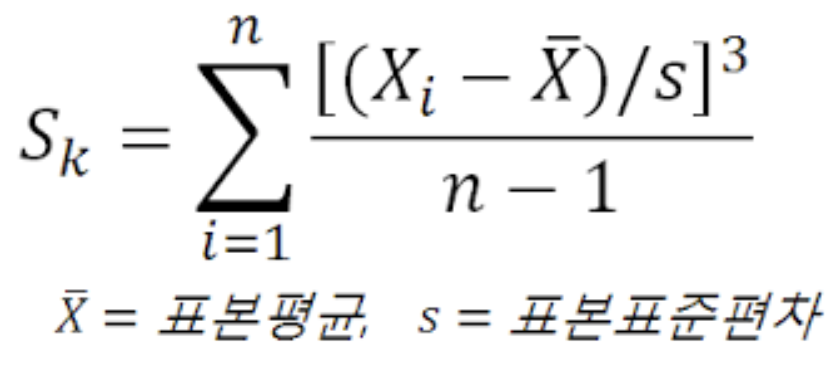
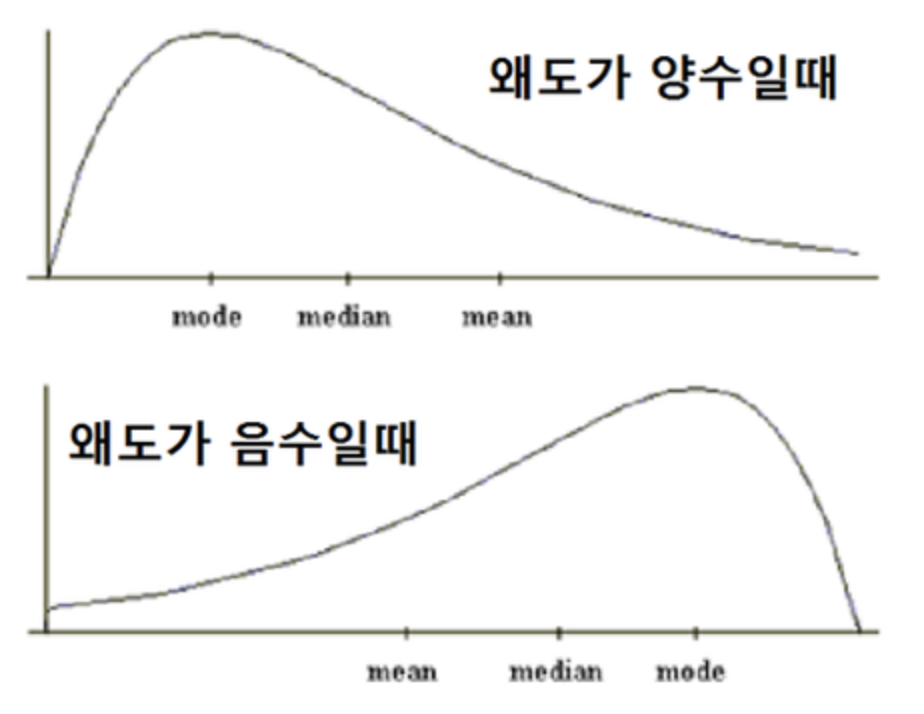
왜도(Skewness) - skew()
1 | > skew1=function(x){ |
nrow(),ncol()- Matrix, data.framelength()- Vector
첨도(Kurtosis) - kurtosi()
1 | > kur=function(x){ |
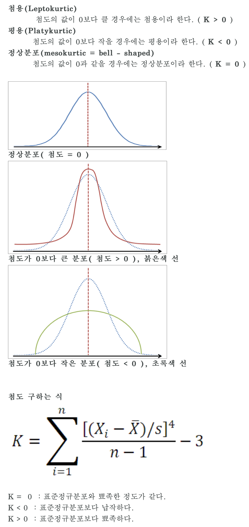
- 정규분포는 왜도가 0 첨도가 3
- 첨도는 기준을 0 or 3 - 이론은 무조건 3 기준
kurtosi() < 3- 완첨kurtosi() = 3- 중첨kurtosi() > 3- 급첨
기술통계학
자료 요약 및 정리 : 표(도수분포표)와 그래프()
범주형 - 도수분포표(빈도를 그래프로 할 수 있긴 함)
수치형 - 기술통계량(분포의 특성)
- 대표값(중심위치)
- 산술평균
- 중위수
- 최빈수(보통 범주형에서 사용, 수치형에선 이산형에서 가끔)
- 산포도(흩어진 정도)
- 표준편차(기존단위가 같음)
- 분산(단위^2)
- 변이(변동)계수(CV) :
sd()/mean() - 사분위수범위(Q3-Q1) :
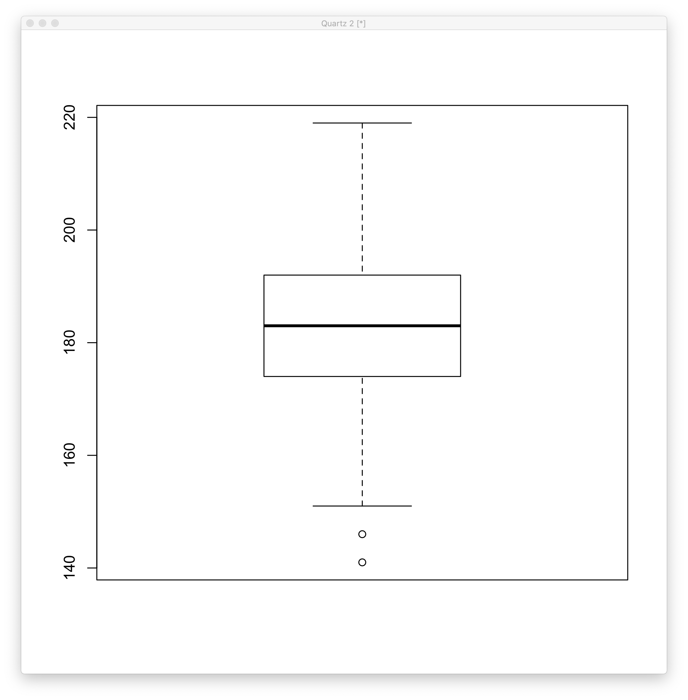
boxplot()
- 비대칭도
- 왜도
- 대표값(중심위치)
오류데이터 찾기
- 최소값
- 최대값
- 도수분포표
summary()
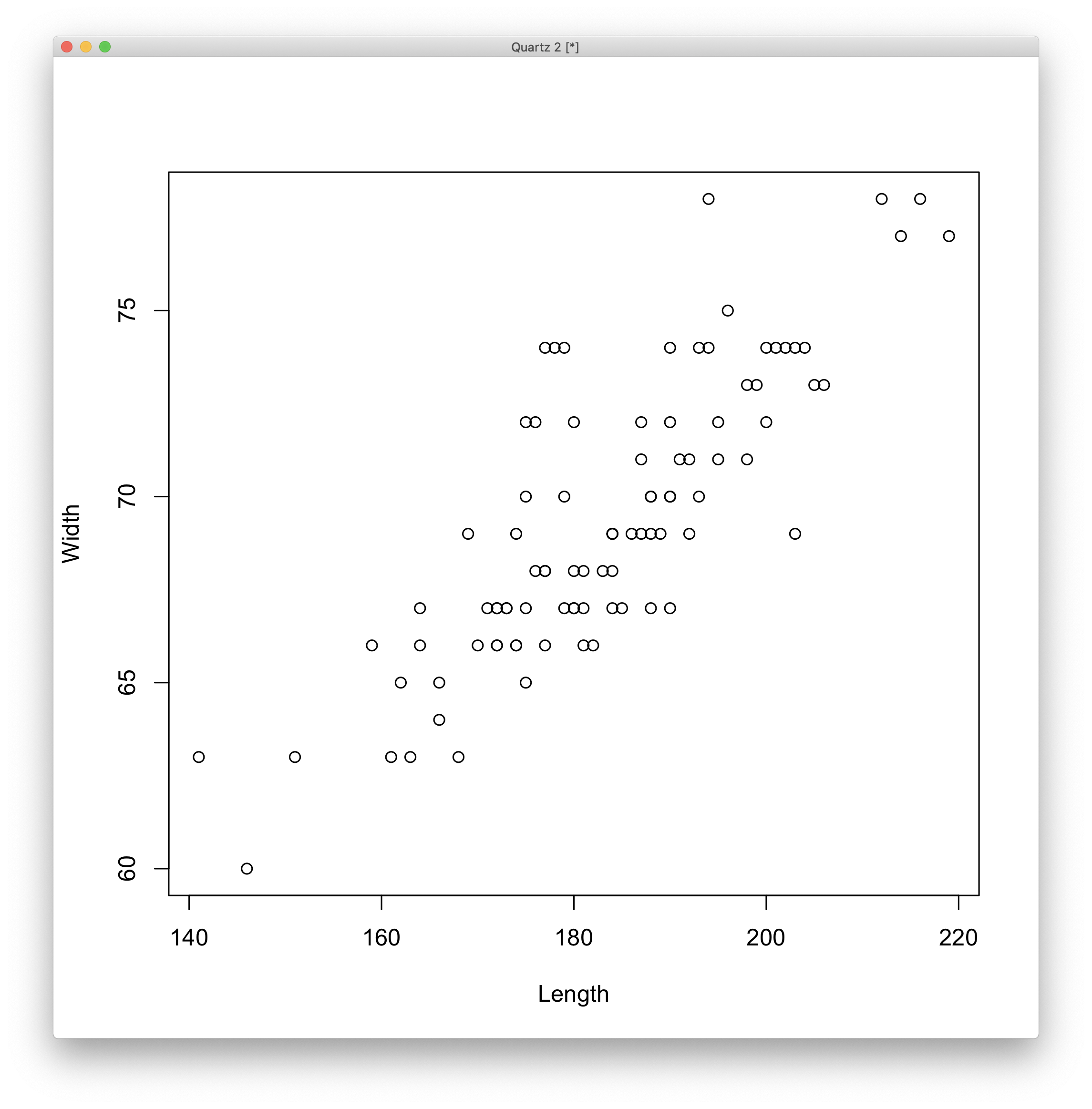
관련된 변수 2개
- 수치형 2개 :
cor(name1,name2) - 범주형 2개 : 교차표(분할표)
- 수치형 2개 :
외부파일 읽기(
.txt) -read.table()/read.csv()-str()-summary()- Data 여러개 - Data handling
- 병합
rbind- 행(Case) 추가cbind- 열(변수) 추가
- 새로운 변수 생성
- 변수계산 : 기존 변수를 가지고 계산을 통해 새로운 변수 생성
- 코딩변경 : 기존 변수를 가지고 새로운 변수 생성(Ex. 학점 예제) - 보통 범주형
- 데이터 취사선택 :
indexing - [],subset() - 정렬 :
sort(),order()
- 병합
- Data 여러개 - Data handling
Slicing :
substr()NA :
mean(name,na.rm=T)출력 :
cat(),sink(),pdf(),dev.off()연산자, 제어문(반복문, 조건문), 함수
단위계산은
*,/만 계산
변동계수
- 평균의 차가 많은 집단끼리의 산포도 비교시 사용
- 단위가 다른 변수에 대한 산포도 비교 - 무차원수
- 극심한 비대칭일때 사용
1 | > boxplot(Length) |
기말
확률변수, 확률분포(이산형, 연속형), 표본분포, 가설검정, 통계분석기법