MATLAB (6)

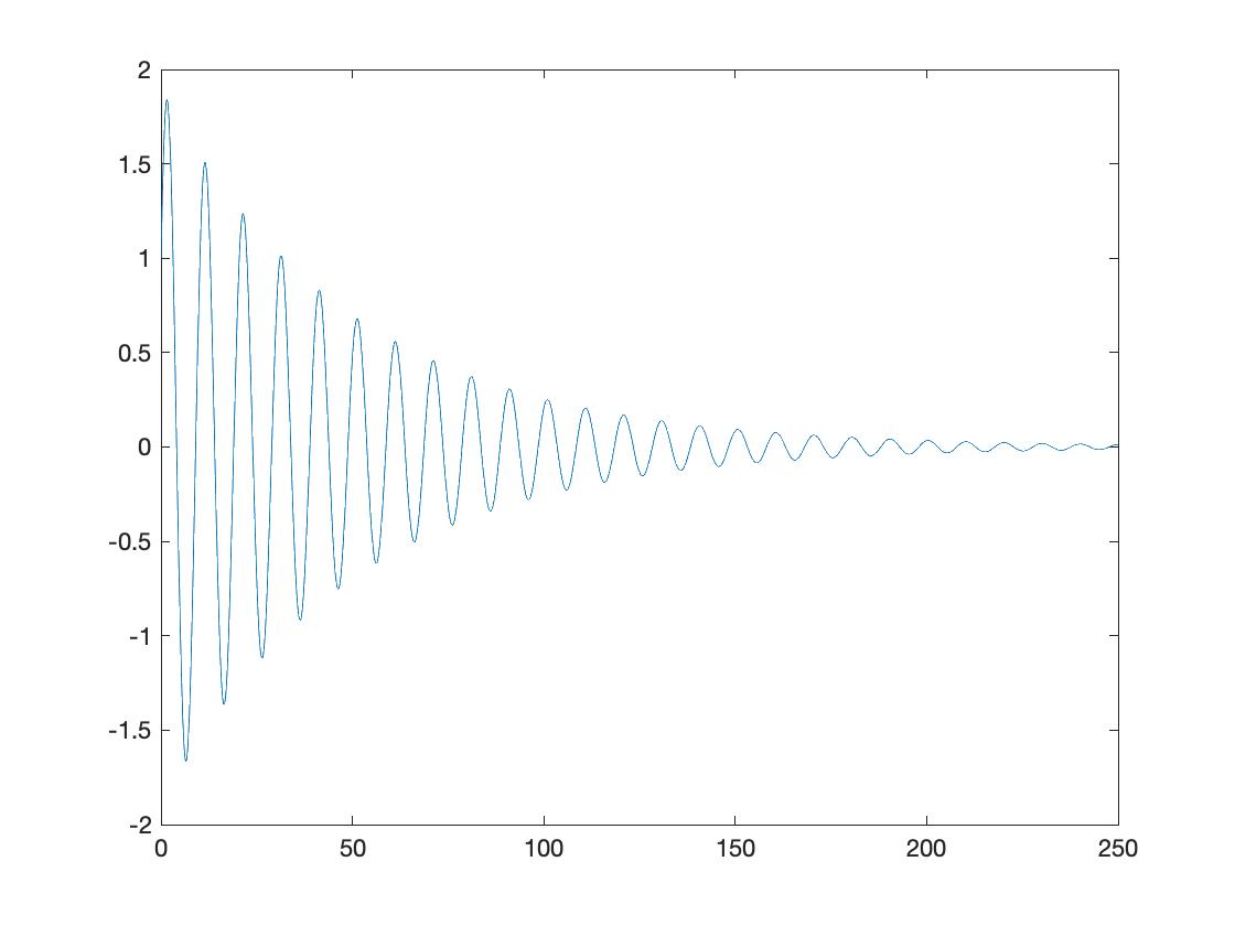
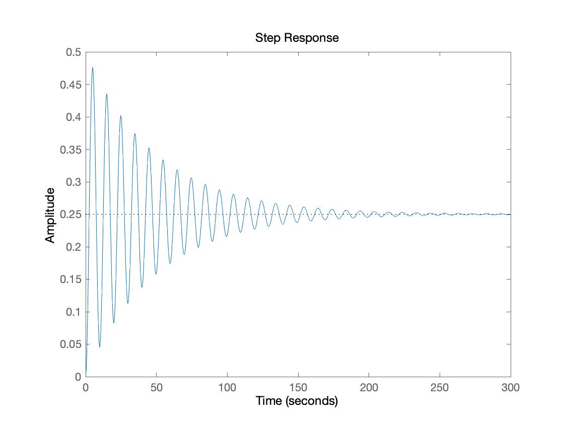
m=10kg, c=0.4Ns/m, k=4Nm(Mass-Spring-Damper System)

General solution, Natural response, Step response

1
2
3
4
5
6
7
8
9
10
11
12
13
14
syms x y;
u=dsolve('D2y+0.04*Dy+0.4*y=0','x')
U=dsolve('D2y+0.04*Dy+0.4*y=0','y(0)=1','Dy(0)=1','x');
subs_U=subs(U,x,0:0.1:250);
t=0:0.1:250;
plot_U=double(subs_U);
plot(t,plot_U)
hold on

figure
num=[1];
den=[10 0.4 4];
h=tf(num, den);
step(h)

General solution

1
2
3
4
5
>> test

u =

C5*exp(-x/50)*cos((3*111^(1/2)*x)/50) - C6*exp(-x/50)*sin((3*111^(1/2)*x)/50)

Natural response
Step response

subs plot

1
2
3
4
subs_U=subs(U,x,0:0.01:10);
t=0:0.01:10;
plot_U=double(subs_U);
plot(t, plot_U)

pole

1
2
3
4
5
6
pole(h)

ans =

-0.0200 + 0.6321i
-0.0200 - 0.6321i

State-space equation

1
2
3
4
5
6
7
8
9
10
11
12
13
14
15
16
17
18
19
20
21
22
[A,B,C,D]=tf2ss(num, den)

A =

-0.0400 -0.4000
1.0000 0


B =

1
0


C =

0 0.1000


D =

0

TF by solve

1
2
3
4
5
6
7
8
9
10
11
12
13
14
15
16
17
18
19
20
21
22
23
24
syms x y;
u=dsolve('D2y+0.04*Dy+0.4*y=0','x')
U=dsolve('D2y+0.04*Dy+0.4*y=0','y(0)=1','Dy(0)=1','x');
subs_U=subs(U,x,0:0.1:250);
t=0:0.1:250;
plot_U=double(subs_U);
plot(t,plot_U)
hold on

syms s t Y;
f=heaviside(t);
Y1=s*Y;
Y2=s*Y1;
sol=solve(10*Y2+0.4*Y1+4*Y-laplace(f),Y);
pretty(sol)
num=[1];
den=[10 0.4 4];
h=tf(num, den);
figure
step(h)

pole(h)

[A,B,C,D]=tf2ss(num, den)
1
2
3
4
5
6
7
8
9
10
11
12
13
14
15
16
17
18
19
20
21
22
23
24
25
26
27
28
29
30
31
32
33
34
35
36
37
38
39
>> test

u =

C3*exp(-x/50)*cos((3*111^(1/2)*x)/50) - C4*exp(-x/50)*sin((3*111^(1/2)*x)/50)

1
---------------------
/ 2 2 s \
s | 10 s + --- + 4 |
\ 5 /


ans =

-0.0200 + 0.6321i
-0.0200 - 0.6321i


A =

-0.0400 -0.4000
1.0000 0


B =

1
0


C =

0 0.1000


D =

0