MATLAB (3)

Mass-Spring-Damper System

1
2
3
4
5
6
7
8
9
10
11
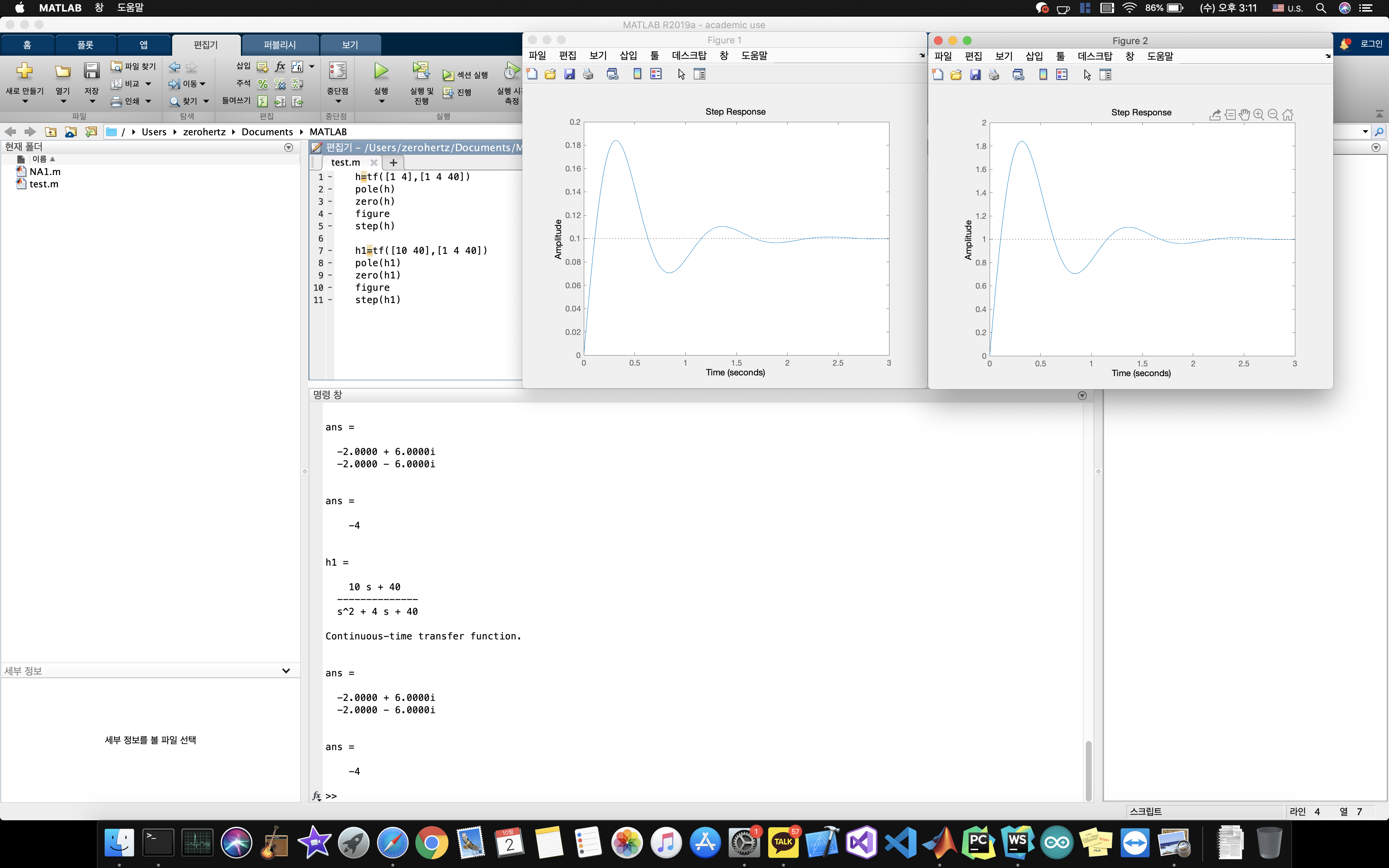
h=tf([1 4],[1 4 40])
pole(h)
zero(h)
figure
step(h)

h1=tf([10 40],[1 4 40])
pole(h1)
zero(h1)
figure
step(h1)

result-1

1
2
3
4
5
6
7
8
9
10
11
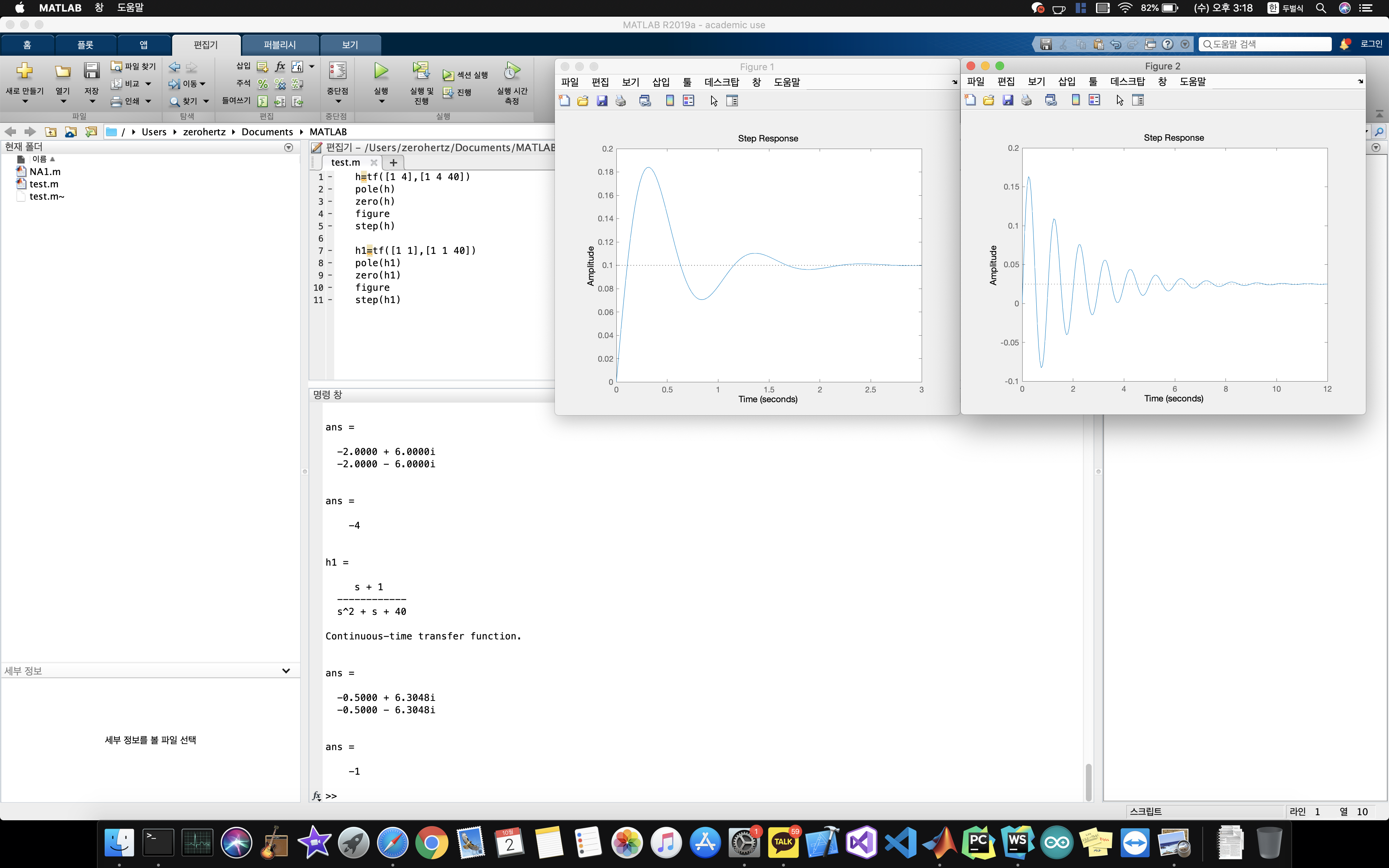
h=tf([1 4],[1 4 40])
pole(h)
zero(h)
figure
step(h)

h1=tf([1 1],[1 1 40])
pole(h1)
zero(h1)
figure
step(h1)

result-2

1
2
3
4
5
6
7
8
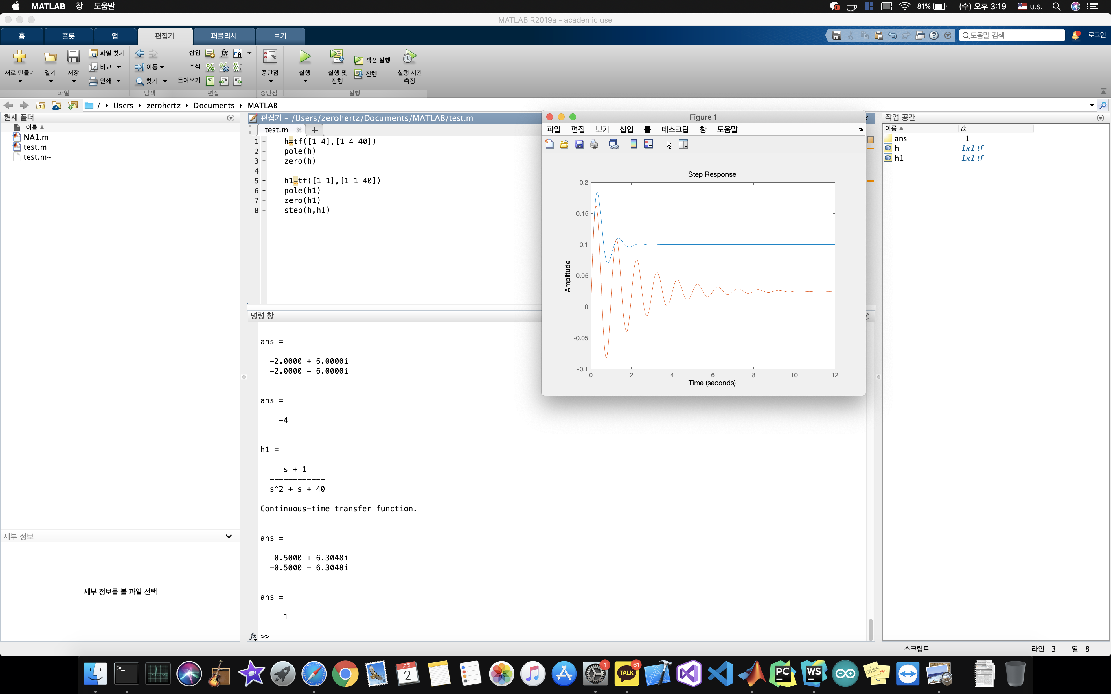
h=tf([1 4],[1 4 40])
pole(h)
zero(h)

h1=tf([1 1],[1 1 40])
pole(h1)
zero(h1)
step(h,h1)

result-3


Value 대입

subs함수 이용

1
2
3
4
5
6
7
8
9
>> help subs
subs - Symbolic substitution

This MATLAB function returns a copy of s, replacing all occurrences of old with
new, and then evaluates s.

subs(s,old,new)
subs(s,new)
subs(s)
1
2
3
4
5
6
7
8
9
10
11
12
13
14
15
16
17
18
syms t y
U1=dsolve('D2y+2*Dy+y=0','y(0)=1','Dy(0)=5','t');
U2=subs(U1,t,0:0.1:10)
U3=double(U2)

U11=dsolve('D2y+2*Dy+2*y=0','y(0)=1','Dy(0)=5','t');
U22=subs(U11,t,0:0.1:10)
U33=double(U22)

U111=dsolve('D2y+2*Dy+3*y=0','y(0)=1','Dy(0)=5','t');
U222=subs(U111,t,0:0.1:10)
U333=double(U222)

figure
plot(U3)
hold on
plot(U33)
plot(U333)
1
2
3
4
5
6
7
8
9
~~~
***
# Laplace transform

> Unit step function

~~~Matlab
syms t
laplace(heaviside(t))
  • 실행결과
1
2
3
ans =

1/s

t^n

1
2
syms t n
laplace(t^n)
  • 실행결과
1
2
3
4
5
6
7
8
9
ans =

piecewise(-1 < real(n) | 1 <= n & in(n, 'integer'), gamma(n + 1)/s^(n + 1))

>> pretty(ans)
{ gamma(n + 1)
{ ------------ if -1 < real(n) or (1 <= n and n in integer)
{ n + 1
{ s

Sin function

1
2
syms t n
laplace(sin(n*t))
  • 실행결과
1
2
3
ans =

n/(n^2 + s^2)

Differential

1
2
3
syms t f(t) s
Df = diff(f(t),t);
laplace(Df,t,s)
  • 실행결과
1
2
3
ans =

s*laplace(f(t), t, s) - f(0)

Inverse Laplace transform

1
2
3
4
5
6
7
8
9
10
11
12
13
14
15
16
17
18
19
20
21
22
23
24
25
26
27
help ilaplace
--- sym/ilaplace에 대한 도움말 ---

ilaplace Inverse Laplace transform.
F = ilaplace(L) is the inverse Laplace transform of the sym L
with default independent variable s. The default return is a
function of t. If L = L(t), then ilaplace returns a function of x:
F = F(x).
By definition, F(t) = int(L(s)*exp(s*t),s,c-i*inf,c+i*inf)
where c is a real number selected so that all singularities
of L(s) are to the left of the line s = c, i = sqrt(-1), and
the integration is taken with respect to s.

F = ilaplace(L,y) makes F a function of y instead of the default t:
ilaplace(L,y) <=> F(y) = int(L(y)*exp(s*y),s,c-i*inf,c+i*inf).

F = ilaplace(L,y,x) makes F a function of x instead of the default t:
ilaplace(L,y,x) <=> F(y) = int(L(y)*exp(x*y),y,c-i*inf,c+i*inf),
integration is taken with respect to y.

Examples:
syms s t w x y f(x)
ilaplace(1/(s-1)) returns exp(t)
ilaplace(1/(t^2+1)) returns sin(x)
ilaplace(t^(-5/2),x) returns (4*x^(3/2))/(3*pi^(1/2))
ilaplace(y/(y^2 + w^2),y,x) returns cos(w*x)
ilaplace(laplace(f(x),x,s),s,x) returns f(x)