
Hands-on Machine Learning (2)
Support Vector Machine (SVM)
- Linear, nonlinear classification
- Regression
- Outlier detection
Linear SVM Classification
- SVM Classifier: 각 클래스 사이에 가장 폭이 넓은 경계 정의 (large margin classification)
- Support vector: 분류기의 경계에 위치한 훈련 데이터
- 분류기의 경계 밖에 훈련 샘플을 더 추가해도 경계가 변화하지 않음
Soft Margin Classification
- Hard margin classification: 모든 샘플이 경계 밖에 올바르게 분류되어 있는 경우
- 데이터가 선형적으로 구분될 수 있어야 정상 작동
- 이상치에 민감하여 일반화가 어려움
- Soft margin classification: 마진 최대화와 마진 오류 (margin violation) 사이에 적절한 균형을 이루는 경우
- Hyperparameter $C$
- Low $C$: 마진 오류 증가, 일반화 성능 향상
- High $C$: 마진 오류 감소, 일반화 성능 감소
- SVM 모델이 과대적합인 경우 $C$를 감소시켜 모델을 규제할 수 있음
- Hyperparameter $C$
1 | import numpy as np |
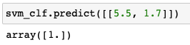
Classification of trained SVM model
Nonlinear SVM Classification
1 | from sklearn.datasets import make_moons |
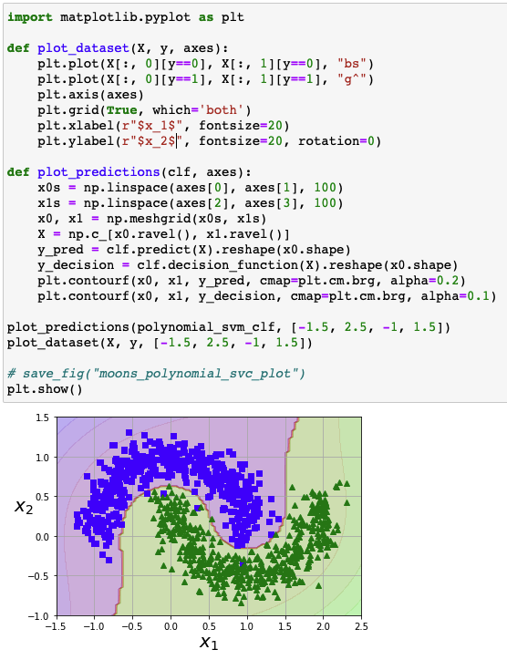
Linear SVM classifier based on polynomial features
Polynomial Kernel
- Polynomial features: 간단하고 다양한 머신러닝 알고리즘에서 적합
- 복잡한 데이터셋에 대해 한계점 존재
- 높은 차수의 다항식이 생성될 경우 모델의 속도 저하 발생
- Kernel trick: 실제로 특성을 추가하지 않고 수학적 전개를 통해 비선형 분류
1 | from sklearn.svm import SVC |
- 3차 다항식 커널 이용
- 모델의 과대적합 발생 $\rightarrow$ 커널의 차수 감소
- 모델의 과소적합 발생 $\rightarrow$ 커널의 차수 증가
coef0: 모델이 높은 차수와 낮은 차수에 얼마나 영향을 받을지 조절하는 hyperparameter
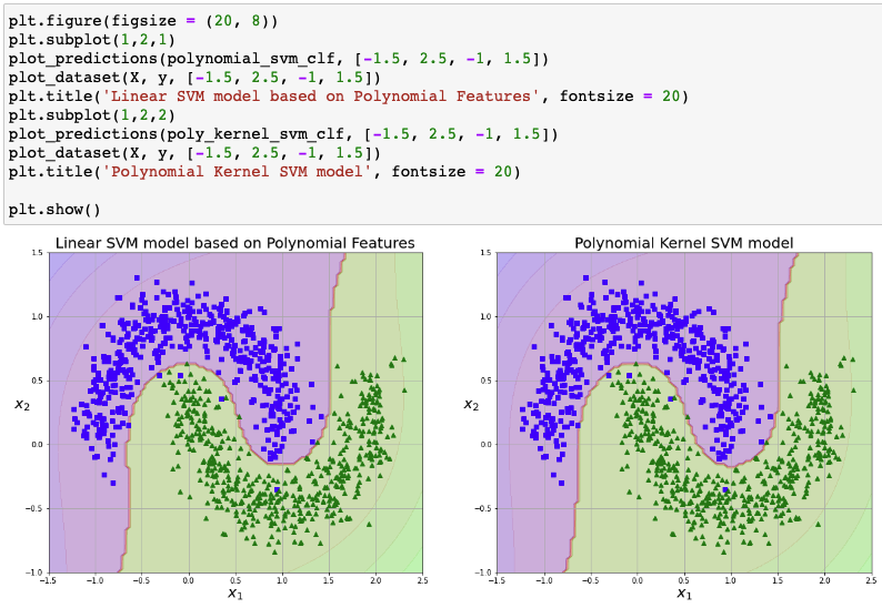
Linear SVM model based on Polynomial Features vs. Polynomial Kernel SVM model
Adding Similarity Features
- 유사도 함수 (similarity function): 각 샘플이 특정 랜드마크와 얼마나 닮았는지 측정
Gaussian RBF (Radial Basis Function)
$$
\phi_\gamma(\boldsymbol{x},l)=\exp{(-\gamma||\boldsymbol{x}-l||^2)}
$$
1 | def gaussian_rbf(x, landmark, gamma): |
Improved linear classification through Gaussian RBF
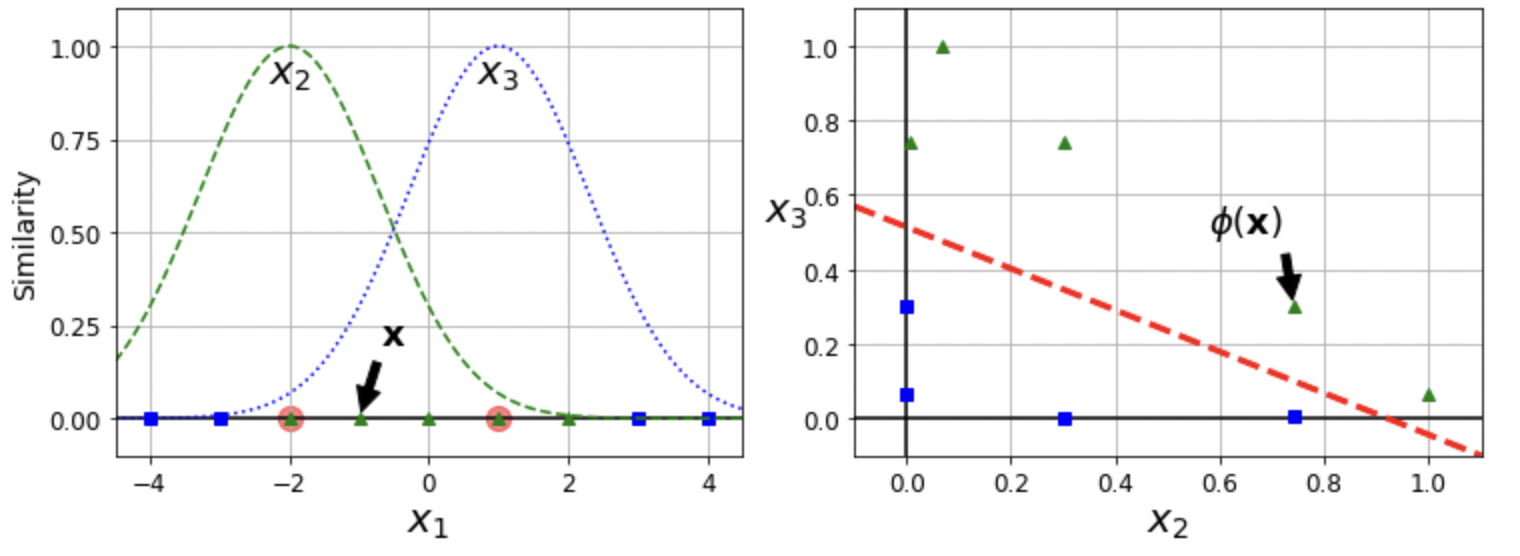
- Landmark: $x_1=-2$ (green), $x_1=1$ (blue)
- Sample $x_1=-1$ $\rightarrow$ $x_2=\exp(-0.3\times1^2)\approx0.74$, $x_3=\exp(-0.3\times2^2)\approx0.30$
- $\gamma = 0.3$
- 훈련 세트의 차원을 수학적으로 확대하여 선형 분류성 향상
Gaussian RBF Kernel
1 | rbf_kernel_svm_clf = Pipeline([ |
Gaussian SVM according to hyperparameters
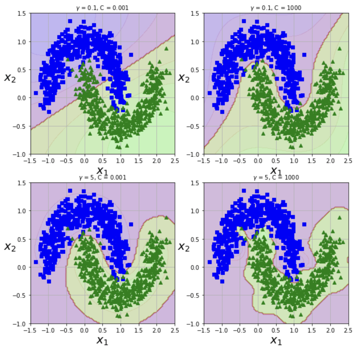
- Hyperparameter $\gamma$
- Low $\gamma$: 결정 경계가 상대적으로 규칙적이고 부드러움
- High $\gamma$: 결정 경계가 상대적으로 불규칙하고 구부러짐
| Class | Time complexity | Out-of-core support | Scaling required | Kernel trick |
|---|---|---|---|---|
| LinearSVC | $O(m\times n)$ | X | O | X |
| SGDClassifier | $O(m\times n)$ | O | O | X |
| SVC | $O(m^2\times n)$ to $O(m^3\times n)$ | X | O | O |
SVM Regression
1 | from sklearn.svm import LinearSVR |
SVM Regression according to hyperparameters
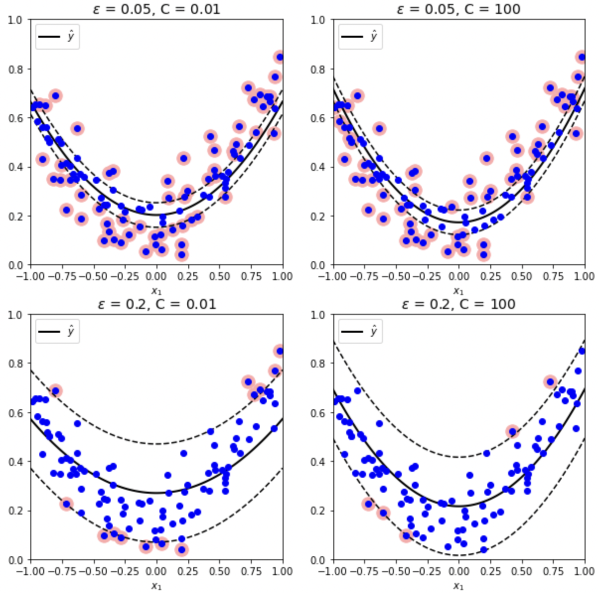
- SVM Regression: 제한된 마진 오류 내에서 마진이 포함하는 샘플 최대화
- Hyperparameter $\varepsilon$: 마진의 폭 설정
- Hyperparameter $C$:
- Low $C$: 마진 오류에 대한 규제 강화 (마진 오류 증가)
- High $C$: 마진 오류에 대한 규제 약화 (마진 오류 감소)
SVM Theory
- Notation
- $\theta_0,\ b$: 편향 (bias)
- $\theta_1$ ~ $\theta_n,\ \boldsymbol{w}$: 가중치 (weight)
- Linear SVM Classifier
- 결정 함수: $\boldsymbol{w}^T\boldsymbol{x}+b=w_1x_1+…+w_nx_n+b$ $\rightarrow$ class prediction
- 결정 함수 $>$ 0: $\hat{y}$ = positive class (1)
- 결정 함수 $\leq$ 0: $\hat{y}$ = negative class (0)
- Training: 설정된 마진의 조건 (하드 마진 / 소프트 마진)을 만족하면서 마진을 최대화 시키는 $\boldsymbol{w},\ b$를 산출해내는 과정
- 목적 함수
- 결정 함수의 기울기 = 가중치 벡터의 노름 ($||\boldsymbol{w}||$)
- $||\boldsymbol{w}||$이 작을수록 마진 증가
- $\therefore$ 마진을 최대화하기 위해 $||\boldsymbol{w}||$ 최소화
- 하드 마진 선형 SVM 분류기의 목적 함수: $\underset{\boldsymbol{w},b}{\operatorname{minimize}}\frac{1}{2}\boldsymbol{w}^T\boldsymbol{w}$ (if $i=1,2,…,m\ \rightarrow\ t^{(i)}(\boldsymbol{w}^T\boldsymbol{x}^{(i)}+b)\geq 1$)
- 소프트 마진 선형 SVM 분류기의 목적 함수: $\underset{\boldsymbol{w},b,\zeta}{\operatorname{minimize}}\frac{1}{2}\boldsymbol{w}^T\boldsymbol{w}+C\Sigma_{i=1}^m\zeta^{(i)}$ (if $i=1,2,…,m\ \rightarrow\ t^{(i)}(\boldsymbol{w}^T\boldsymbol{x}^{(i)}+b)\geq 1-\zeta^{(i)},\ \zeta^{(i)}\geq0$)
- 결정 함수: $\boldsymbol{w}^T\boldsymbol{x}+b=w_1x_1+…+w_nx_n+b$ $\rightarrow$ class prediction
- Kernel SVM
- Linear: $K(\boldsymbol{a,b})=\boldsymbol{a}^T\boldsymbol{b}$
- Polynomial: $K(\boldsymbol{a,b})=(\gamma\boldsymbol{a}^T\boldsymbol{b}+r)^d$
- Gaussian RBF: $K(\boldsymbol{a,b})=\exp{(-\gamma||\boldsymbol{a}-\boldsymbol{b}||^2)}$
- Sigmoid: $K(\boldsymbol{a,b})=\tanh{\gamma\boldsymbol{a}^T\boldsymbol{b}+r}$
Decision Tree
- Classification
- Regression
- Multioutput tasks
Training and Visualization
1 | from sklearn.tree import DecisionTreeClassifier |
Visualization
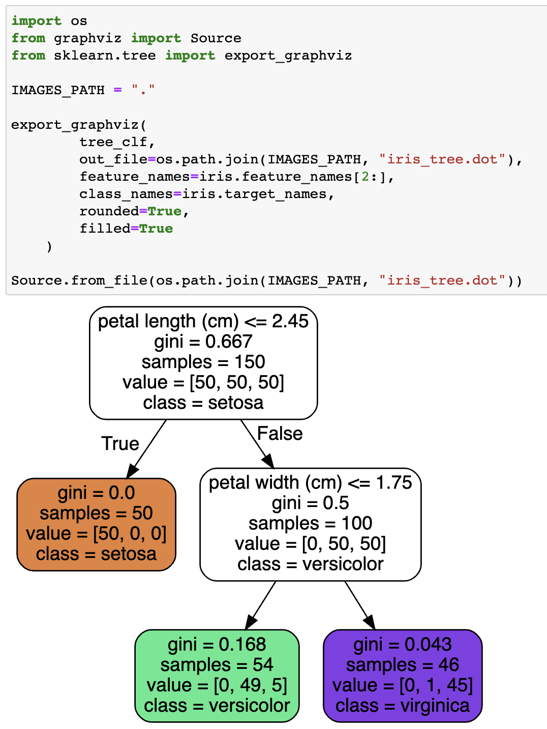
Prediction
- Root node: 깊이가 0인 최상위 노드
- Leaf node: Child node를 가지지 않는 노드
- Gini: 불순도 (impurity) 측정 값
- 모든 샘플이 같은 클래스 $\rightarrow$ gini = 0
Gini impurity
$$
G_i=1-\Sigma^n_{k=1}p_{i,k}^2
$$
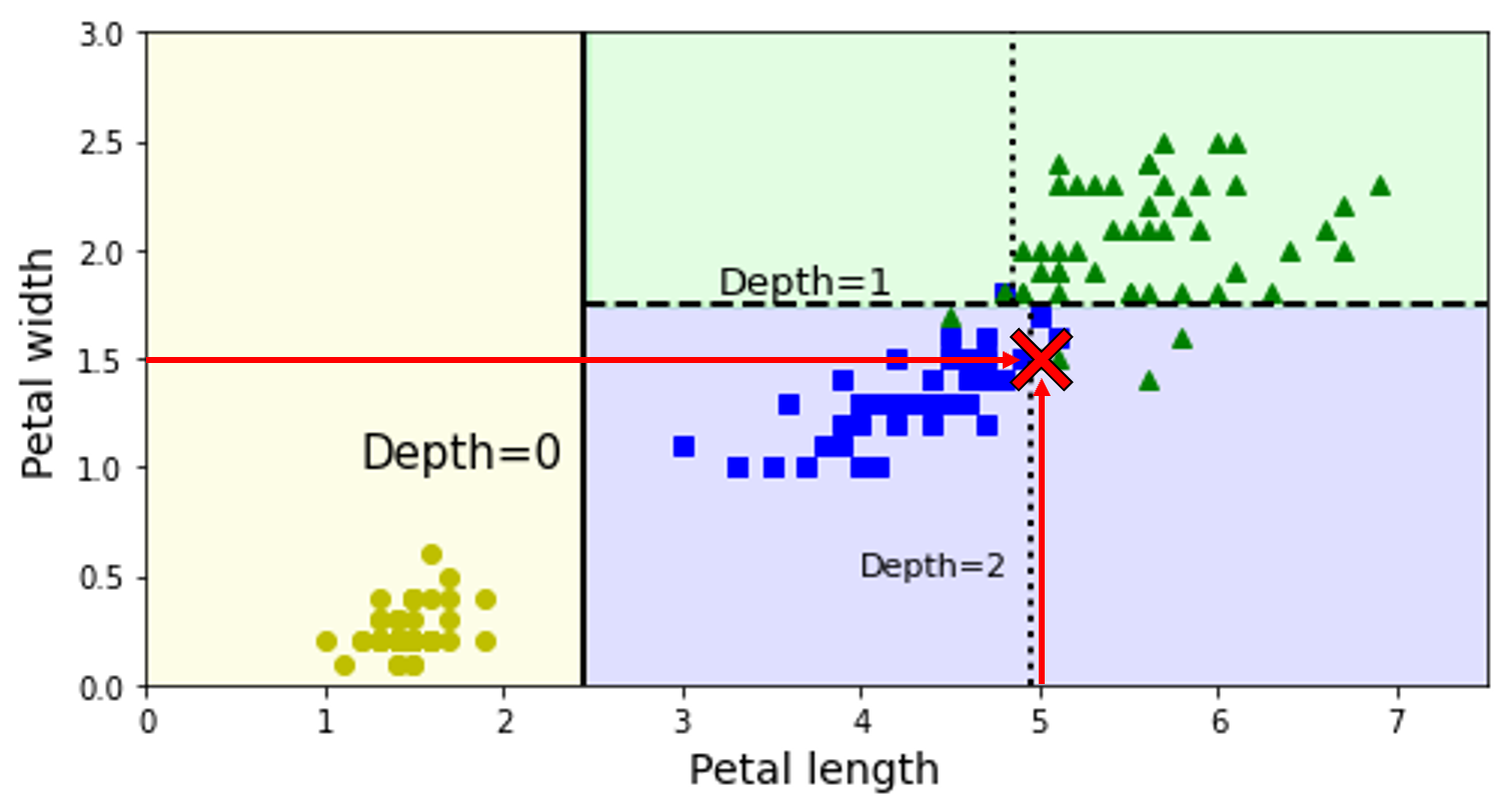
Decision boundaries
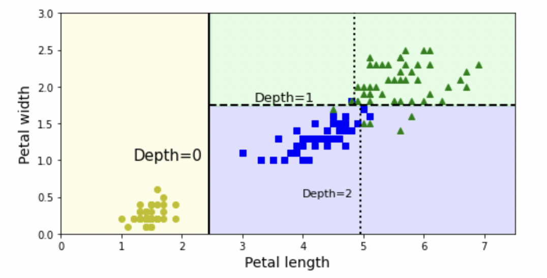
Estimating Class Probabilities
Class estimation process
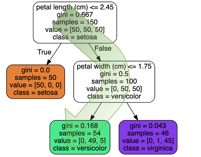
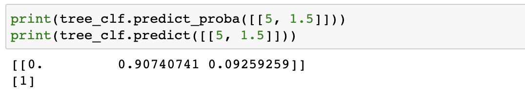
- $0\%=0/54\times100$
- $90.7\%=49/54\times100$
- $9.3\%=5/54\times100$
CART Training Algorithm
- CART (Classification And Regression Tree)
- 하나의 특성 $k$의 임계값 $t_k$를 사용하여 두개의 서브셋으로 나눔
- 하단의 비용 함수 최소화 (가장 순수한 서브셋으로 나눌 수 있는 $(k,t_k)$ 짝 도출)
- 나누어진 서브셋에 대해 최대 깊이 만큼 위의 절차 반복 (불순도 감소 불가 시 정지)
CART cost function for classification
$$
J(k,t_k)=\frac{m_{left}}{m}G_{left}+\frac{m_{right}}{m}G_{right}
$$
- $G_{left/right}$: 좌측/우측 서브셋의 불순도
- $m_{left/right}$: 좌측/우측 서브셋의 샘플 수
Computational Complexity
결정 트리를 탐색하기 위한 계산 복잡도
$$
O(\log_2(m))
$$
각 노드에서 모든 훈련 샘플의 모든 특성 비교 시 계산 복잡도
$$
O(n\times m\log_2(m))
$$
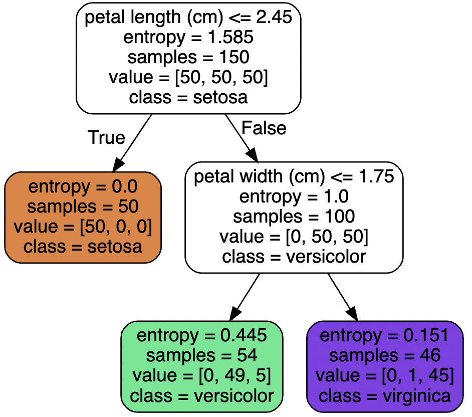
Entropy Impurity
criterion = "entropy": 지니 불순도 대신 엔트로피 불순도 사용- 한 서브셋 내의 모든 샘플의 클래스가 동일 $\rightarrow\ H_i=0$
- Vs. Gini Impurity
- 큰 차이는 존재하지 않음
- 지니 불순도의 계산 속도
- 다른 트리가 만들어 질 때 엔트로피가 더 균형잡힘
$$
H_i=-\overset{n}{\underset{p_{i,k}\neq0}{\underset{k=1}{\Sigma}}} p_{i,k}\log_2(p_{i,k})
$$
Entropy Impurity
Regularization Hyperparameters
- Nonparametric model (비파라미터 모델): 훈련되기 전 파라미터의 수가 결정되지 않는 모델 (과대적합 위험 존재)
- Parametric model (파라미터 모델): 모델 파라미터의 수가 미리 정의 (과소적합 위험 존재)
- Regularization hyperparameter (규제 매개변수): 훈련 데이터에 대한 과대적합을 피하기 위해 학습할 때 모델의 자유도 제한
DecisionTreeClassifiermax_depth: 결정 트리의 깊이 (기본값 =None, 제한 없음)min_samples_split: 분할되기 위해 노드가 가져야하는 최소 샘플 수min_samples_leaf: 리프 노드가 가지고 있어야할 최소 샘플 수min_weight_fraction_leaf: 가중치가 부여된 전체 샘플 수에서의 비율max_leaf_nodes: 리프 노드의 최대 수max_features: 각 노드에서 분할에 사용할 특성의 최대 수
Regression
1 | from sklearn.tree import DecisionTreeRegressor |
Decision Tree Regression
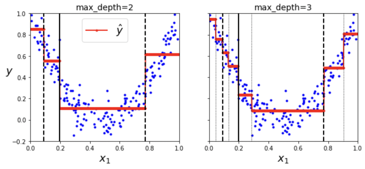
- 각 노드에서 값 예측
- 각 영역의 예측값은 그 영역에 있는 훈련 데이터의 평균
CART cost function for regression
$$
J(k,t_k)=\frac{m_{left}}{m}MSE_{left}+\frac{m_{right}}{m}MSE_{right}
$$
- $MSE_{node}=\underset{i\in node}{\Sigma}(\hat{y}_{node}-y^{(i)})^2$
- $\hat{y}_{node}=\frac{1}{m_{node}}\underset{i\in node}{\Sigma}y^{(i)}$
Limitation
훈련 데이터의 회전과 작은 변화에 민감 $\rightarrow$ Random Forest 모델을 통해 개선