
Hands-on Machine Learning (1)
Setting up development environment
Clone source code
Ref: Hands-on Machine Learning
1 | git clone https://github.com/rickiepark/handson-ml2.git |
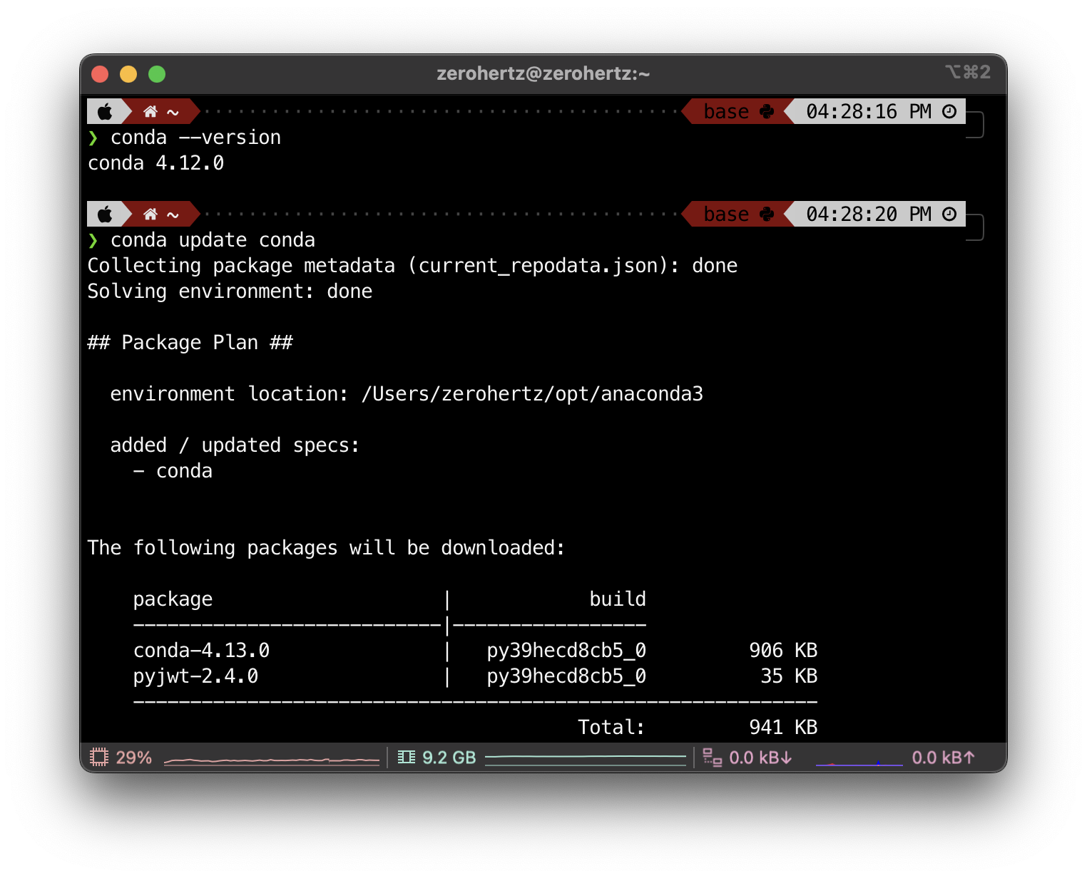
Download Anaconda
1 | conda --version |
Download Jupyter Notebook
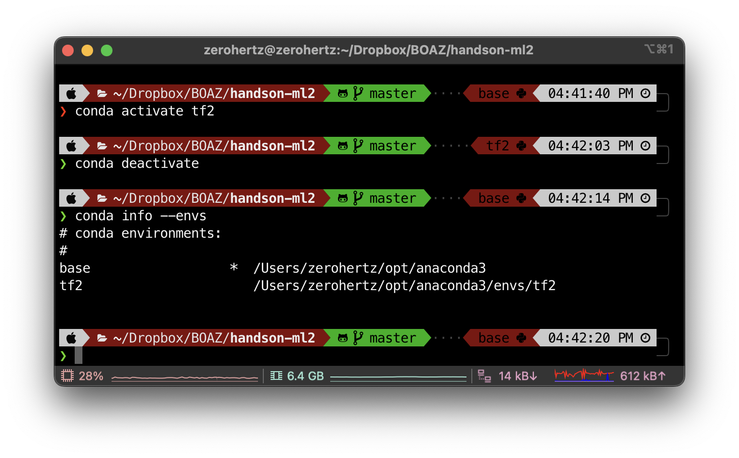
Set environment
1 | conda env create -f environment.yml |
1 | jupyter notebook |
Setting complete

Machine Learning
Definition of Machine Learning: The science (and art) of programming computers so they can learn from data
- Supervised Learning: The training data you feed to the algorithm includes the desired solutions, called
labels- Classification
- k-Nearest Neighbors (kNN)
- Linear Regression
- Logistic Regression
- Support Vector Machines (SVM)
- Decision Trees and Random Forests
- Neural Networks
- Regression
- k-Nearest Neighbors (kNN)
- Linear Regression
- Logistic Regression
- Support Vector Machines (SVM)
- Decision Trees and Random Forests
- Neural Networks
- Classification
- Unsupervised Learning: The training data is unabled
- Clustering
- K-Means
- DBSCAN
- Hierarchical Cluster Analysis (HCA)
- Anomaly detection and novelty detection
- One-class SVM
- Isolation Forest
- Visualization and dimensionality reduction
- Principal Component Analysis (PCA)
- Kernel PCA
- Locally-Linear Embedding (LLE)
- t-distributed Stochastic Neighbor Embedding (t-SNE)
- Association rule learning
- Apriori
- Eclat
- Clustering
- Semi-supervised Learning: Dealing with partially labeled training data, usually a lot of unlabeled data and a little bit of labeled data
- Deep Belief Networks (DBNs)
- Restricted Boltzmann Machines (RBMs)
- Reinforcement Learning: How intelligent agents ought to take actions in an environment in order to maximize the notion of cumulative reward
Classification
Training a Binary Classifier
1 | from sklearn.linear_model import SGDClassifier |
Performance Measures
Confusion Matrix
| Predicted: Negative | Pridicted: Positive | |
|---|---|---|
| Actual: Negative | True Negative (TN) | False Positive (FP) |
| Actual: Positive | False Negative (FN) | True Positive (TP) |
1 | from sklearn.model_selection import cross_val_predict |
$$
precision = \frac{TP}{TP + FP}
$$
1 | from sklearn.metrics import precision_score |
$$
recall = \frac{TP}{TP + FN}
$$
1 | from sklearn.metrics import recall_score |
$$
F_1 = 2\times\frac{precision\times recall}{precision+recall}
$$
1 | from sklearn.metrics import f1_score |
Precision and recall versus the decision threshold (precision/recall tradeoff)
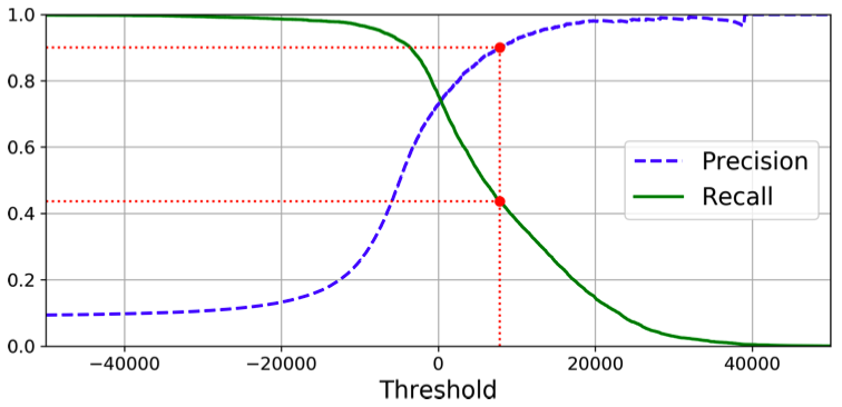
1 | from sklearn.metrics import precision_recall_curve |
ROC (Receiver Operating Characteristic) curve
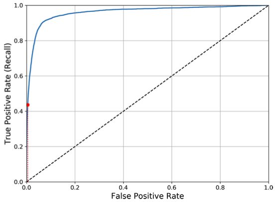
1 | from sklearn.metrics import roc_curve |
ROC AUC (Area Under the Curve)
1 | from sklearn.metrics import roc_auc_score |
Multiclass Classification
One-versus-All (OvA)
- $N$ Classifiers
1 | sgd_clf.fit(X_train, y_train) |
One-versus-One (OvO)
- $N\times(N-1)/2$ Classifiers
1 | from sklearn.multiclass import OneVsOneClassifier |
Scaling the inputs
1 | from sklearn.preprocessing import StandardScaler |
Error Analysis
1 | y_train_pred = cross_val_predict(sgd_clf, X_trained_scaled, y_train, cv = N) |
Multioutput Classification
1 | knn_clf.fit(X_train, y_train) |
Training Models
Linear Regression
Linear regression model prediction
$$
\hat{y}=\theta_0+\theta_1x_1+\theta_2x_2+…+\theta_nx_n
$$
- $\hat{y}$: Predicted value
- $n$: The number of features
- $x_i$: The $i^{th}$ feature value
- $\theta_j$: The $j^{th}$ model parameter
Mean Square Error (MSE) cost function for a linear regression model
$$
MSE(\boldsymbol{X}, h_{\boldsymbol{\theta}})=\frac{1}{m}\Sigma^m_{i=1}(\boldsymbol{\theta}^T\boldsymbol{x}^{(i)}-y^{(i)})^2
$$
Gradient Descent
Partial derivatives of the cost function
$$
\frac{\partial}{\partial\theta_j}MSE(\boldsymbol{\theta})=\frac{2}{m}\Sigma^m_{i=1}(\boldsymbol{\theta}^T\boldsymbol{x}^{(i)}-y^{(i)})x^{(i)}_j
$$
Gradient vector of the cost function
$$
\nabla_{\boldsymbol{\theta}}MSE(\boldsymbol{\theta})=\frac{2}{m}\boldsymbol{X}^T(\boldsymbol{X\theta-y})
$$
Gradient descent step
$$
\boldsymbol{\theta}^{(next\ step)}=\boldsymbol{\theta}-\eta\nabla_{\boldsymbol{\theta}}MSE(\boldsymbol{\theta})
$$
Polynomial Regression
1 | from sklearn.preprocessing import PolynomialFeatures |
Ridge Regression
Ridge regression cost function
$$
J(\boldsymbol{\theta})=MSE(\boldsymbol{\theta})+\alpha\frac{1}{2}\Sigma^n_{i=1}\theta_i^2
$$
1 | from sklearn.linear_model import Ridge |
Lasso Regression
Lasso regression cost function
$$
J(\boldsymbol{\theta})=MSE(\boldsymbol{\theta})+\alpha\Sigma^n_{i=1}|\theta_i|
$$
1 | from sklear.linear_model import Lasso |
Elastic Net
Elastic net cost function
$$
J(\boldsymbol{\theta})=MSE(\boldsymbol{\theta})+r\alpha\Sigma^n_{i=1}|\theta_i|+\frac{1-r}{2}\alpha\frac{1}{2}\Sigma^n_{i=1}\theta_i^2
$$
1 | from sklearn.linear_model import ElasticNet |
Logistic Regression
Logistic regression model estimated probability
$$
\hat{p}=h_{\boldsymbol{\theta}}(\boldsymbol{x})=\sigma(\boldsymbol{x}^T\boldsymbol{\theta})
$$
Logistic function
$$
\sigma(t)=\frac{1}{1+e^{-t}}
$$
Logistic regression cost function (log loss)
$$
J(\boldsymbol{\theta})=-\frac{1}{m}\Sigma^m_{i=1}[y^{(i)}log(\hat{p}^{(i)})+(1-y^{(i)})log(1-\hat{p}^{(i)})]
$$
1 | from sklearn.linear_model import LogisticRegression |
Softmax Regression
Softmax score for class $k$
$$
s_k(\boldsymbol{x})=\boldsymbol{x}^T\boldsymbol{\theta}^{(k)}
$$
Softmax function
$$
\hat{p}_k=\sigma(\boldsymbol{s}(\boldsymbol{x}))_k=\frac{exp(s_k(\boldsymbol{x}))}{\Sigma^K_{j=1}exp(s_j(\boldsymbol{x}))}
$$
- $K$: The number of classes
- $\boldsymbol{s}(\boldsymbol{x})$: A vector containing the scores of each class for the instance $\boldsymbol{x}$
- $\sigma(\boldsymbol{s}(\boldsymbol{x}))_k$: The estimated probability that the instance $\boldsymbol{x}$ belongs to class $k$ given the scores of each class for that instance
Softmax regression classifier prediction
$$
\hat{y}=\underset{k}{\operatorname{arg max}}\sigma(\boldsymbol{s}(\boldsymbol{x}))_k=\underset{k}{\operatorname{arg max}}s_k(\boldsymbol{x})=\underset{k}{\operatorname{arg max}}((\boldsymbol{\theta}^{(k)})^T\boldsymbol{x})
$$
Cross entropy cost function
$$
J(\boldsymbol{\Theta})=-\frac{1}{m}\Sigma^m_{i=1}\Sigma^K_{k=1}y_k^{(i)}log(\hat{p}_k^{(i)})
$$
- $y_k^{(i)}$: The target probability that the $i^{th}$ instance belongs to class $k$
Cross entropy gradient vector for class $k$
$$
\nabla_{\boldsymbol{\theta}^{(k)}}J(\boldsymbol{\Theta})=\frac{1}{m}\Sigma^m_{i=1}(\hat{p}_k^{(i)}-y_k^{(i)})\boldsymbol{x}^{(i)}
$$