Generative Adversarial Network (1)
PyTorch
Setup
How to install PyTorch in M1 Mac
1 | conda install pytorch torchvision torchaudio -c pytorch-nightly |
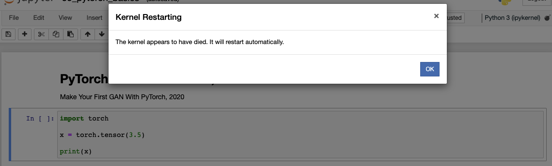
conda activate env이후jupyter notebook을 통해import torch를 실행할 경우 위의 사진과 같이 커널이 죽는다.- 따라서 아래 명령어를 통해
jupyter notebook에서 커널을 선택할 수 있게 해줘야한다.
1 | conda install nb_conda_kernels |
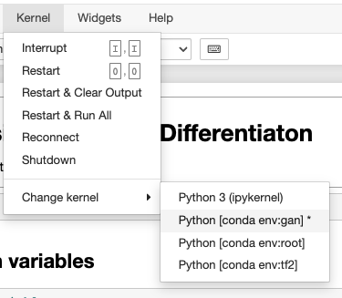
- 위의 모듈
nb_conda_kernels를 통해 모든 가상환경들을 선택해서jupyter notebook에서 사용할 수 있다.
Tensor and Gradient
1 | x = torch.tensor(3.5) |
1 | tensor(3.5000) tensor(5.5000) |
- 일반적 계산과 다르게
PyTorch내에서의 수식은 $y(x) = x$와 같이 저장된다.
1 | x = torch.tensor(4., requires_grad = True) |
1 | tensor(17., grad_fn=<AddBackward0>) |
- 이와 같이 $y(x) = x$로 관계가 저장되기 때문에 $y’(x)$를 산정할 수 있다.
1 | x = torch.tensor(4., requires_grad = True) |
1 | tensor(24.) |
- 매개변수와 같은 응용도 가능하다.
- 이 외의 tensor handling
Neural Network based on PyTorch
Data Description (MNIST)
Download MNIST Train Data
Download MNIST Test Data
Read MNIST Data
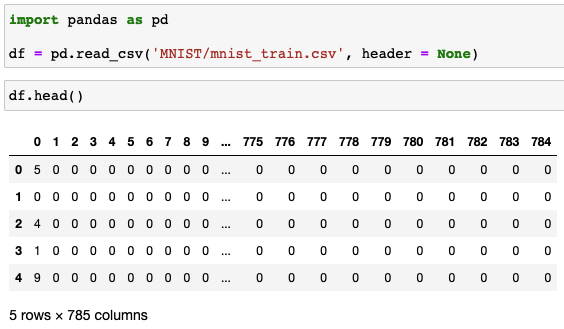
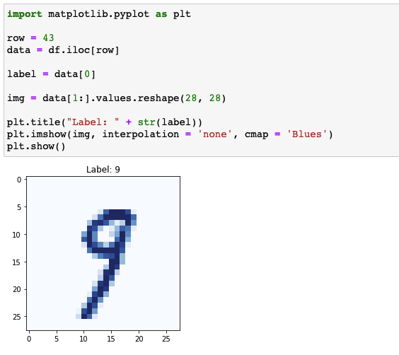
- 첫 숫자는 해당 이미지의 label을 의미한다.
- 나머지 784개의 숫자는 $28\times 28$으로 이뤄진 이미지의 각 픽셀 값이다.
Data Visualization
Artificial Neural Network
- 앞서 말한 것과 같이 이미지는 $28\times 28$ 즉, 784개의 픽셀 값으로 이루어져있다.
- 따라서 input layer는 784개의 node를 지녀야한다.
- 또한 label의 종류가 10개 (0 ~ 9) 이므로 output layer는 10개의 node를 지녀야한다.
- 가장 간단한 신경망을 구성하기 위해 아래 항들을 따른다.
- 특정 layer의 모든 node들은 그 다음 레이어의 모든 node와 연결 (fully connected)
- Input layer와 output layer 사이에 존재하는 hidden layer의 크기는 200
- Hidden layer와 output layer 사이의 activation function은 logistic function
1 | import torch |
| 문법 | 명칭 | 의미 |
|---|---|---|
ANN(nn.Module) |
클래스 이름 | nn.Module로부터 상속 |
__init__() |
생성자 (constructor) | - |
super.__init__() |
- | 부모 클래스의 생성자 호출 |
nn.Sequential() |
- | 파라미터를 통해 간단한 레이어 정의 |
nn.Linear(m,n) |
- | m개의 노드로부터 n개의 노드까지의 선형 완전 연결 매핑 |
nn.Sigmoid() |
- | 로지스틱 활성화 함수를 이전 레이어의 출력에 적용 |
nn.MSELoss() |
- | 신경망에서 오차를 정의하는 방법 중 하나 |
torch.optim.SGD() |
- | 손실을 토대로 신경망의 가중치를 수정하는 방법 중 하나 |
nn.Linear(): $Ax+B$와 같은 형태로 노드 사이를 연결- $A$: 가중치
- $B$: 편향 (bias)
- 위 두 파라미터를 학습 파라미터 (learnable parameter)라고 명함
nn.MSELoss(): 평균제곱오차 (Mean Squared Error)을 통해 실제와 예측된 결과 사이의 차이를 제곱하고 평균내어 계산- Loss function: 학습 파라미터 업데이트하기 위해 오차 계산
- Error (오차) vs. Loss (손실)
- Error: 정답과 예측값 사이의 차이
- Loss: 궁극적으로 풀어야 할 문제에 대한 오차
- 비슷하지만 딥러닝에서 굳이 따지자면 Loss를 기반으로 신경망의 가중치 업데이트
torch.optim.SGD(): 확률적 경사 하강법 (Stochastic Gradient Descent)self.parameters()를 통해 세세한 설정 가능
ANN.forward()- 입력값을 받아
nn.Sequential()에서 정의한self.model()에 전달 - 모델의 결과는
forward()를 호출한 곳으로 전달
- 입력값을 받아
1 | ... |
ANN.train(): 구성한 신경망의 훈련을 위한 메서드- 신경망에 전달할 입력과 원하는 목표의 출력으로 구성 $\rightarrow$ 손실 계산
self.forward(inputs)$\rightarrow$self.model(inputs)$\rightarrow$outputs- 입력값을 신경망에 전달하여 결과 산출
outputs$\rightarrow$self.loss_function()$\rightarrow$loss- 신경망의 손실 계산
self.optimiser.zero_grad()$\rightarrow$loss$\rightarrow$loss.backward()$\rightarrow$self.optimiser.step()- 계산 그래프의 기울기 초기화 후 손실을 통해 신경망의 가중치 업데이트
- 기울기 초기화 제외 시
loss.backward()를 따라 모든 계산에 중첩
Training Process Visualization
1 | ... |
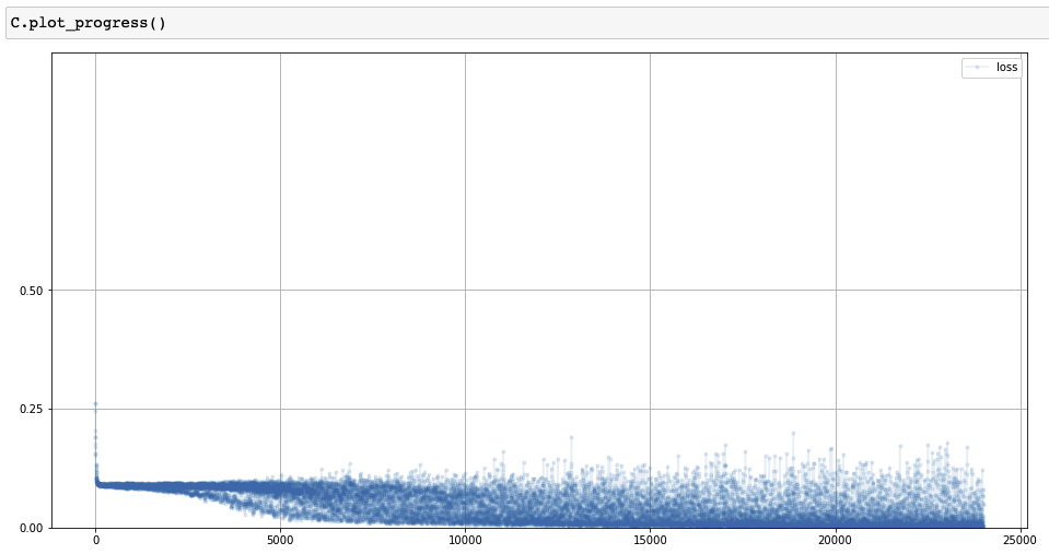
- 훈련이 진행되는 동안 매 10개의 훈련 샘플마다 손실값을 저장하여 시각화
Data Handling for PyTorch
torch.utils.data.Dataset객체 이용
1 | from torch.utils.data import Dataset |
| 문법 | 의미 |
|---|---|
__len__() |
데이터셋의 길이 반환 |
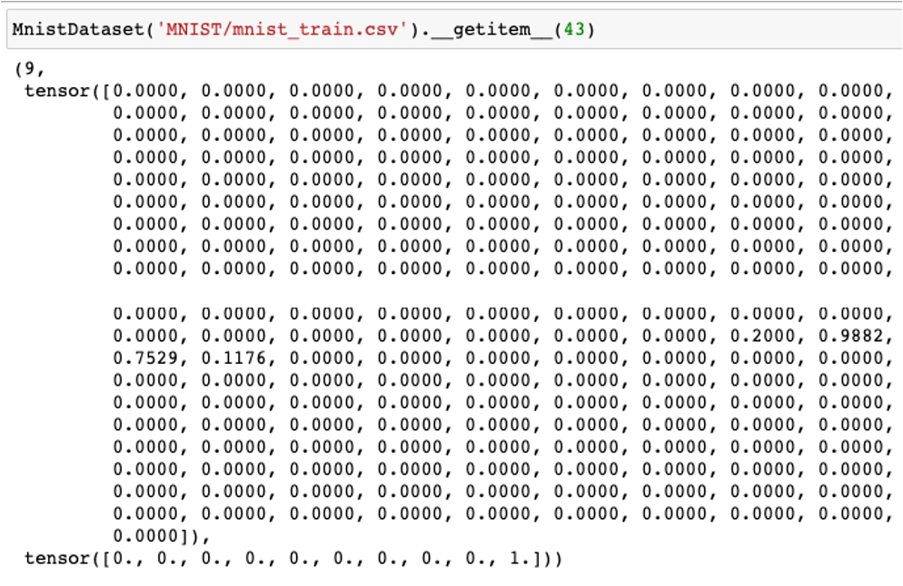
__getitem__() |
데이터셋의 n번째 아이템 반환 |
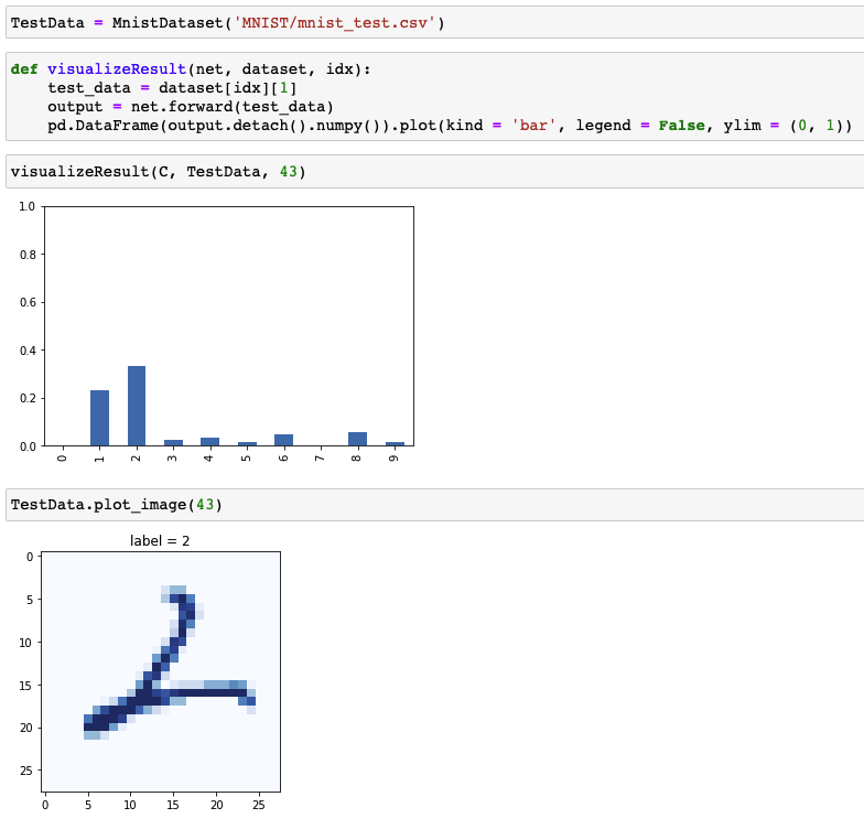
__getitem__()
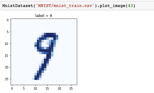
plot_image()
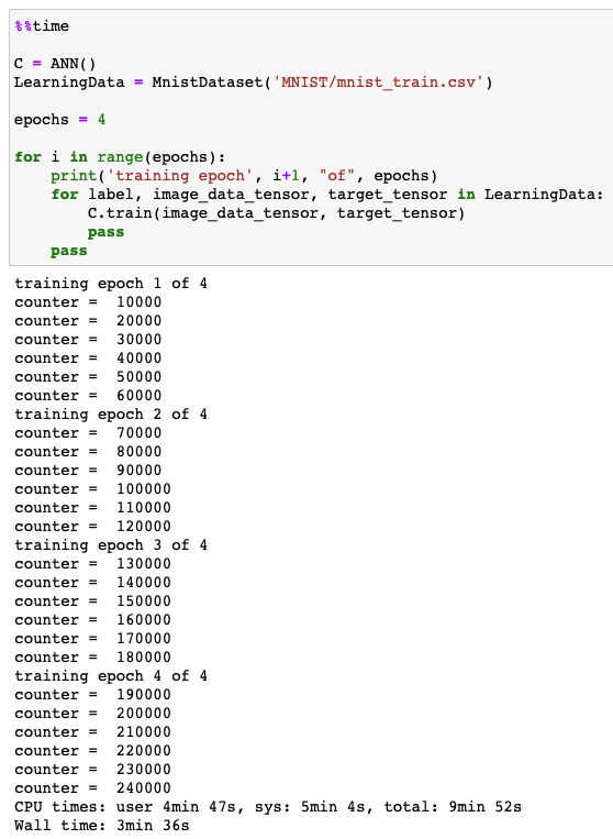
Classifier Training
Classifier training
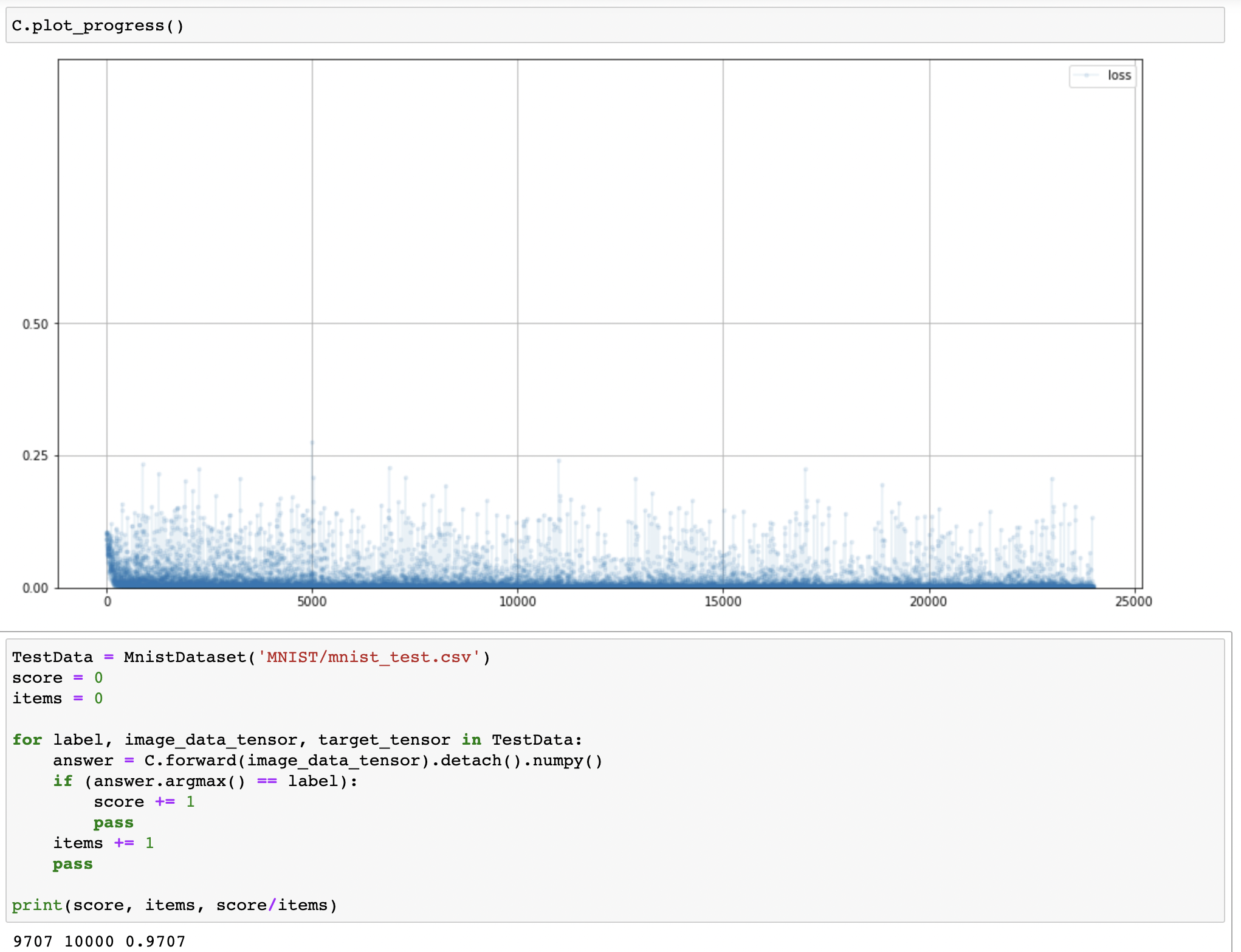
Plot loss chart
Classifier Validation
Classification of test data
Classifier validation
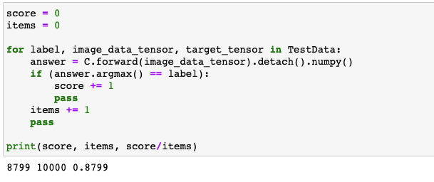
- 87.99%의 분류 정확도
GPU 가속
1 | import torch |
- 근데 CPU로 훈련하는게 더 빠름…
Neural Network Reinforcement
Loss Function
1 | ... |
Reinforcing Neural Network by Changing Loss Function
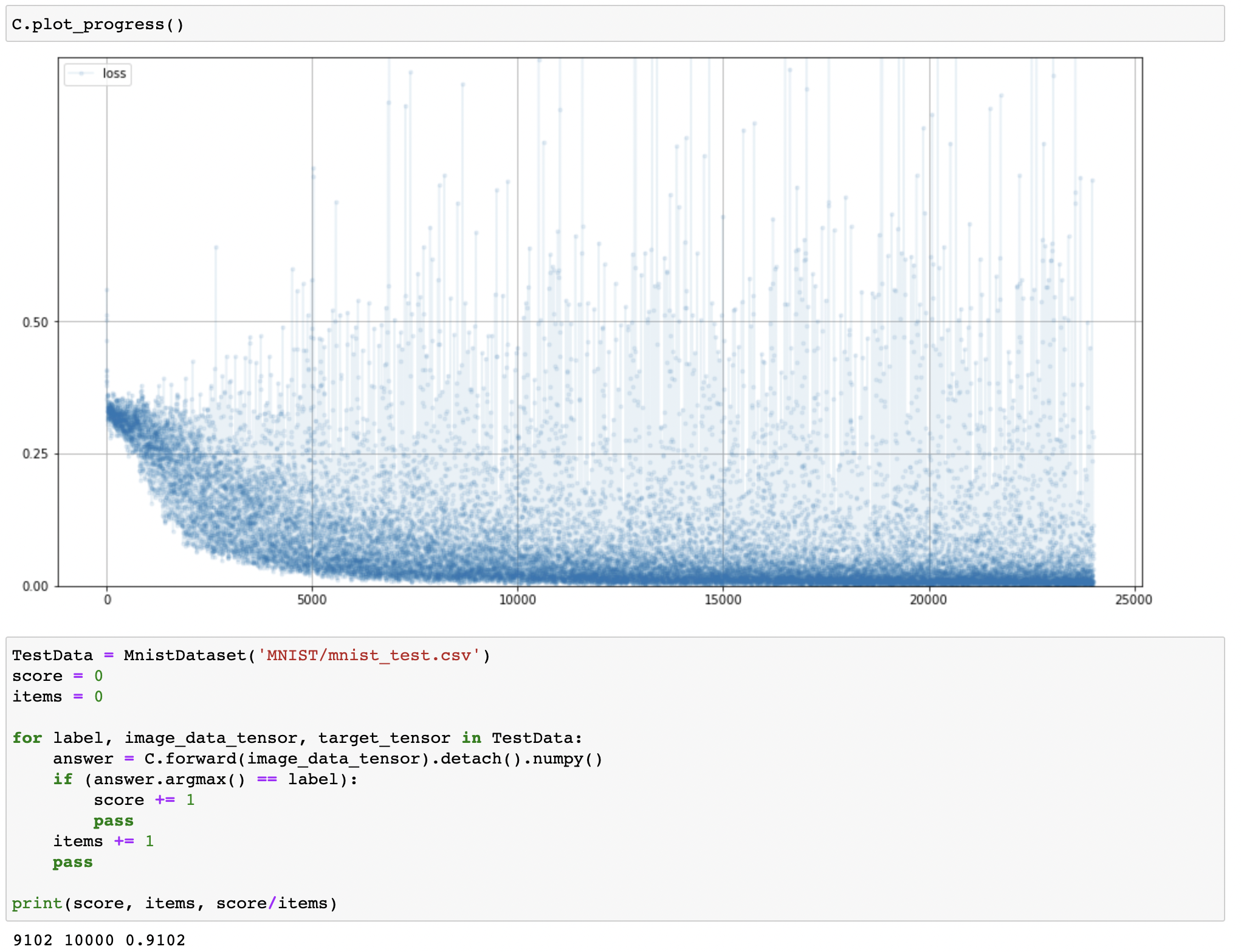
- 이진 교차 엔트로피 (Binary Cross Entropy, BCE) 손실: Classification에서 loss function으로 자주 사용
- 확실하게 틀린 경우 큰 페널티 부여
MSELoss()에 비해 반복에 따라 손실이 느리게 감소BCELoss()을 사용함으로MSELoss()를 사용한 모델에 비해 87.99%에서 91.02%으로 분류 정확도 향상
Activation Function
1 | ... |
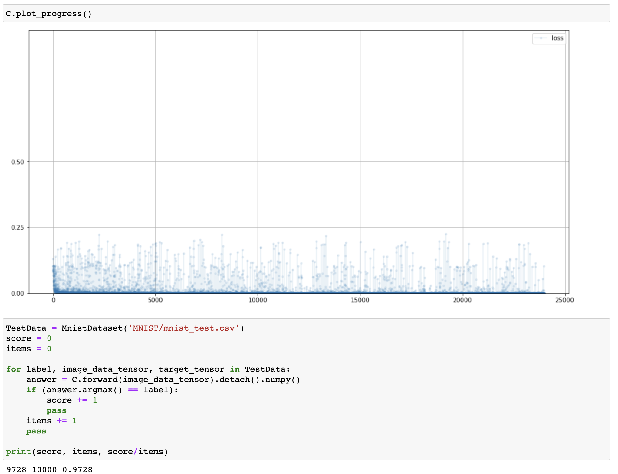
Reinforcing Neural Network by Changing Activation Function
- Logistic function: 뉴런에서 일어나는 신호 전달 현상과 비슷하여 초기의 신경망에서 자주 사용
- 수학적으로 기울기를 도출하기 간단
- 큰 값들에 대해 기울기가 작고 사라질 수 있음
- 소실될 경우 이를 포화 (saturation)이라고 함
- 정류 선형 유닛 (Rectified Linear Unit, ReLU)
- 0보다 큰 값들에 대해 일정한 기울기
- 0보다 작은 값들에 대해 경사가 0이기 때문에 기울기가 소실되는 문제가 여전히 존재
- Leaky ReLU
- 0보다 작은 경우 미세한 기울기 허용
- 손실 함수로
BCELoss()사용 불가 $\rightarrow$ BCE 손실은 0과 1 사이 외의 값을 받을 수 없음 - 91.02%에서 97.07%으로 분류 정확도 향상
Optimizer
1 | ... |
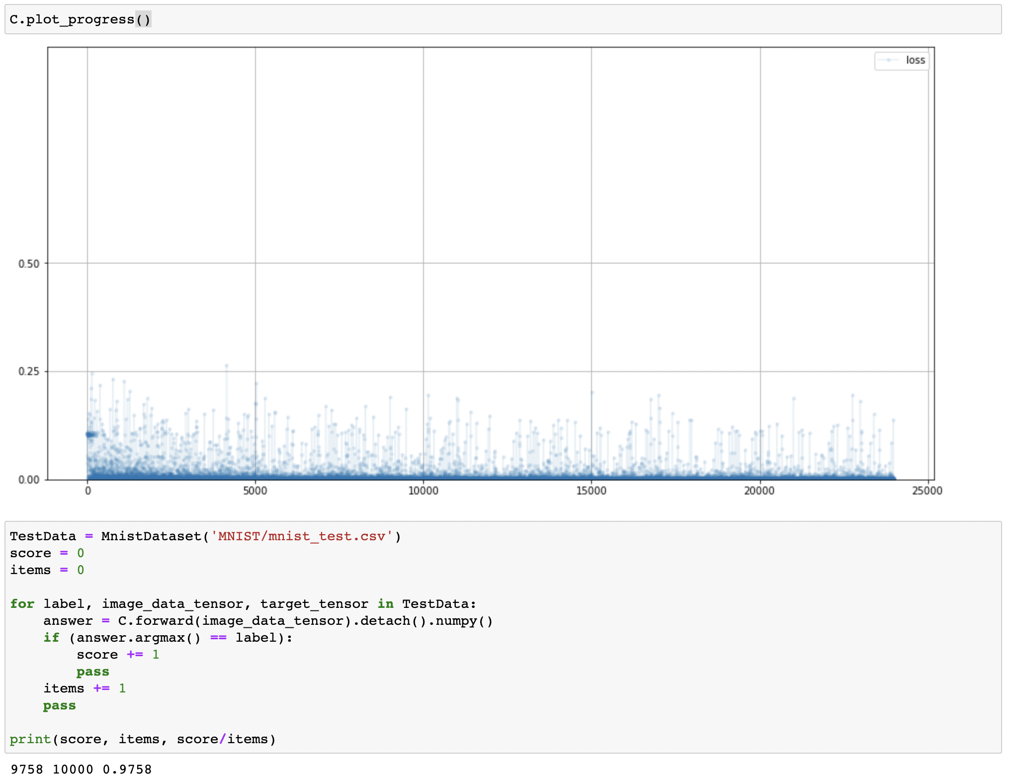
Reinforcing Neural Network by Changing Optimizer
- 확률적 경사 하강법 (Stochastic Gradient Descent, SGD)
- 국소 최적해에 빠질 가능성 존재
- 모든 학습 파라미터에 단일한 학습률 적용
- Adam
- 관성을 이용하여 국소 최적해로 빠질 가능성 최소화
- 각 학습 파라미터에 대해 다른 학습률 적용
Normalization
1 | ... |
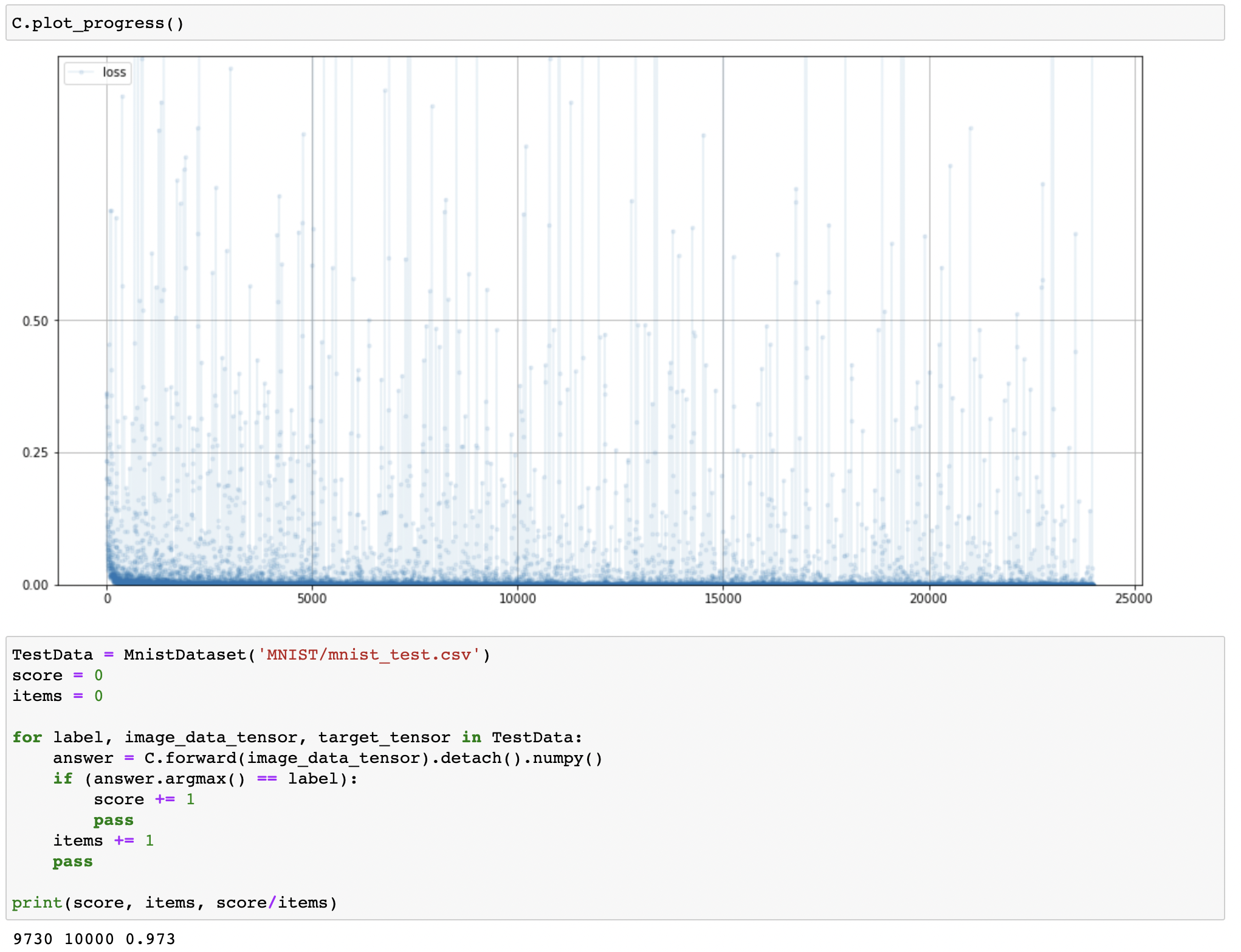
Reinforcing Neural Network by Normalization
- 신경망의 가중치 혹은 신호의 값에 대해 peak로 인해 중요한 값이 소실될 수 있음
- 따라서 파라미터들의 범위를 조절하거나 평균을 0으로 설정하는 방법 사용 $\rightarrow$ 정규화 (normalization)
Combination
1 | ... |
Reinforcing Neural Network
- Loss Function
- Activation Function
- Optimizer
- Normalization
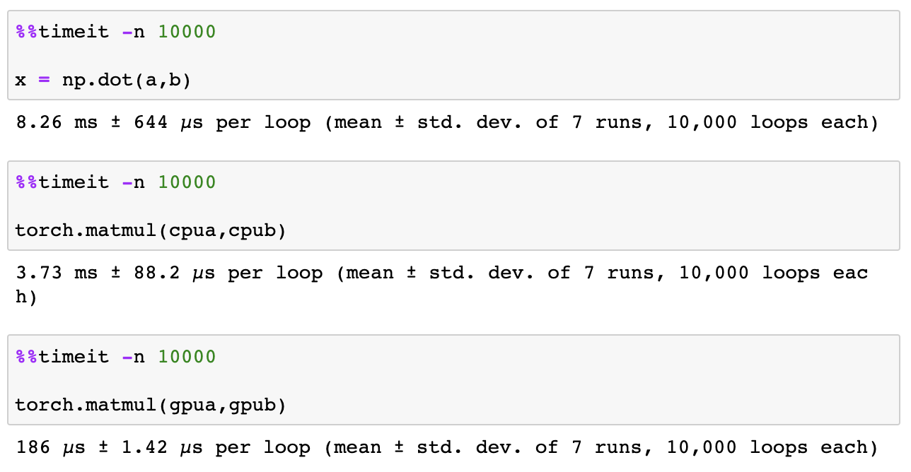
CUDA
- Tensor operation speed: Vanila python <<< Numpy
- CUDA (Compute Unified Device Architecture): GPU (Graphic Processing Unit) 기반 머신러닝 표준 소프트웨어 프레임워크
1 | device = torch.device("mps") #CUDA 아님. . . |
CUDA는 아니지만 M1 Mac에서의 GPU 가속…